

The US Forest Service's Northern Research Station develops & communicates science in 20 Northeast and Midwest states for managing healthy, productive forests.
- Tweets28.3K
- Following1.1K
- Followers13.5K
- Likes1.5K






ALT Tom Schultz, USDA Forest Service Chief with Cindi West, Director of Forest Products Laboratory and Northern Research Station; National Forest Foundation Board members and Forest Service staff gather in the lobby of the Forest Products Laboratory and Northern Research Station headquarters ahead of a laboratory tour. USDA Forest Service photo by Ellie Lazarcik.


ALT Figure 1.—Updated quantitative silviculture tools for the spruce-fir forest type in the Northeast. Panel A is a density management diagram showing combinations of stem density (x-axis) and average stand diameter (y-axis) in five zones of density management space. Panel B presents the same information as a stocking guide, with basal area on the y-axis and average stand diameter rendered as isolines (3 to 17 inches). These graphs are based on work by Ray et al. (2023).

ALT Technological advances, such as the use of passenger drones, could improve recreational access to remote public lands and carry firefighters to hard-to-reach areas. 3D rendering image of a passenger drone. Licensed image by chesky/AdobeStock.

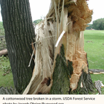
ALT A cottonwood tree broken in a storm urban forests in the conterminous United States. The index . USDA Forest Service photo by Joseph Obrien/Bugwood.org

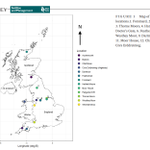
ALT FIGURE 1 Map of the study locations.1. Forsinard, 2. Auchencorth, 3. Thorne Moors, 4. Hatfield Moors, 5. Doctor's Gate, 6. Featherbed, 7. Whixall, 8. Westhey Moor, 9. Dartmoor, 10. Bodmin, 11. Moor House, 12. Chat Moss, and 13. Cors Erddreiniog.

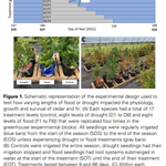
ALT Figure 1. Schematic representation of the experimental design used to test how varying lengths of flood or drought impacted the physiology, growth and survival of cedar and fir. (A) Each species had a total of 17 treatment levels (control, eight levels of drought [D1 to D8] and eight levels of flood [F1 to F8]) that were replicated four times in the greenhouse (experimental blocks). All seedlings were regularly irrigated (blue bars) from the start of the season (SOS) to the end of the season (EOS) unless experiencing drought or flood treatments (gray bars).


ALT Fig. 1. Tapestry Urbanization categories at the Census block group level (A), residential tree canopy cover change (B), yard-level polygons derived from parcels (C). Panels B and C refer to the location of red star in panel A. (For interpretation of the references to colour in this figure legend, the reader is referred to the web version of this article.)

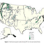
ALT Figure 1—Total forest ecosystem carbon density (MT C ha-1) for each national forest.

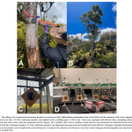
ALT Fig. 1. The efficacy of a commercial verbenone product was tested on ʻohi ¯ ʻa (Metrosideros polymorpha) trees in the field, and the emission of the active ingredient was measured over time

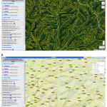
ALT Figure 1.—Base map display including satellite imagery (A) and topographic map (B).

ALT FIGURE 5 | Invasion history of North American A. glabripennis populations. MA, Massachusetts; OH, Ohio; Far, Farmingdale, New York; TOR: Toronto; N1, North Plain region one; N2, North Plain region two; NW, Northwest; NE, Northeast; S, South. Each native region is colored individually, while all invasive populations are in red. Invasive populations experienced a bottleneck event (dashed line) followed by population expansion (solid line). The unsampled ancestry population is shown in black.

ALT Figure 2. Conceptual representation of upper soil and deep soil in a forest system and the key differences between the distinct but connected soil layers related to SOC cycling

ALT FIGURE 1 Fungal necromass loss (%) with different particle size by microbial strain. (A) necromass loss (%) at 14 days post-inoculation (dpi) (solid circle) and 28 (hollow circle) dpi. Control panel shows the percentage of mass loss in uninoculated necromass.

ALT Table 1 Format and structure of the Great Lakes User Group kick-off workshop at Kemp Natural Resources Station, Woodruff, Wisconsin September 2023

ALT Fig. 8. Example meta-modeling approach using a more detailed model to derive tree species growth parameters for a forest landscape model.


ALT FIGURE 2 Numbers of nonnative species discovered (proxy for establishment) each decade from 1850 to 2020.

ALT FIGURE 2 The biogeographic regions where commodities transporting insect predators and parasitoids to the United States were imported from, and the percentage of interceptions arriving from each region. Biogeographic regions were delineated based on the distributions and phylogenetic turnover of amphibian, bird, and mammal species (Holt et al., 2013).

ALT FIGURE 1 | Workflow for modelling tree assemblages and predicting compositional change in response to climate change.