

quant finance, econometrics, regression.
Joined March 2021
- Tweets129
- Following192
- Followers447
- Likes118



One cannot simply copy skills and local context and recreate research taste…yet.
I think probably though that gap will eventually be closed. It feels like it could be “solved” for the most rational aspects of the human condition (math, engineering, industry)
How will nth order models handle the less rational aspects of the spiritual technology [humanity] that the universe manifested, like love, shame, admiration? What even IS existentialism anymore?

Weekend for me is the time for making AI-based artifacts. Very briefly, I
1 write down a problem/open question;
2 pose it to GPT6.1 and Opus5.5 agents, with maximum effort, interacting on common files, using my skills
3 read [some of] the output
4 refine the question
The output is not AI slop (at least, I learn from it) but it's not not AI slop either. It's quite good overall and I learn from them. I wonder if people would be interested in them. Below is an example. Let me know, I don't want to add to the sloppiness in the world.


Nick Patterson (Renaissance Technologies)
"[...I joined a hedged fund, Renaissance Technologies, I'll make a comment about that. It's funny that I think the most important thing to do on data analysis is to do the simple things right. So, here's a kind of non-secret about what we did at renaissance: in my opinion, our most important statistical tool was simple regression with one target and one independent variable. It's the simplest statistical model you can imagine. Any reasonably smart high school student could do it. Now we have some of the smartest people around, working in our hedge fund, we have string theorists we recruited from Harvard, and they're doing simple regression. Is this stupid and pointless? Should we be hiring stupider people and paying them less? And the answer is no. And the reason is nobody tells you what the variables you should be regressing [are]. What's the target. Should you do a nonlinear transform before you regress? What's the source? Should you clean your data? Do you notice when your results are obviously rubbish? And so on. And the smarter you are the less likely you are to make a stupid mistake. And that's why I think you often need smart people who appear to be doing something technically very easy, but actually usually not so easy.]"
1. news.ycombinator.com/item?id…
2. robohub.org/talking-machines…
Kyle Murphy retweeted

1/n
Okay back to regularly scheduled programming. Related to the last thread I wrote up about robustness in portfolio optimization, today we are going to look at a comparison of two types of factor models: a global equity model and an integrated factor model.
Specifically, we will cover the content of 3 papers spanning the use of risk models in: 1) forecasting risk and 2) optimizing portfolios and methods of assessing and comparing models across those two domains.
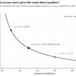
What's the signal share of a short, noisy record, and what is left of it after estimation, constraints, and governance?
Long-only managers in "ouroboros" territory.
The more concentrated the index, the less of it the small stocks hold, so the less room there is to fund overweights without cutting the mega stocks. The bet gets bigger as the mega stocks win and get larger so it feeds on itself.
Hold the top 10 stocks at exactly their index weight and you have taken them out of the game. The rest of the stocks now have to balance among themselves under the same rule. The small end still ends up being overweight and the biggest stocks still allowed to move (11 through 100) pay for it.
Gotta cut big to buy small. The bet just moves down in tiers - doesn't go away.

Further - the shape that picks the uncertainty set picks the shrinkage and that shape matters.
1. In the below post the "opponent's" charge was the distance multiplied by the sum of squared weights. That charge is smallest at equal weight, so it nudges every portfolio toward equal weight. A nudge only helps if it points toward the true answer.
2. W.r.t @0xFaust12's toy example: the nudge points at the truth. All 20 assets are identical so equal weight is the true min-var portfolio. A bigger distance means a harder nudge toward the truth. In this toy example, true risk falls at every step in every history.
3. Given a mixed menu the nudge can point the wrong way. Real menus mix calm and wild assets. We build a different toy: 20 assets with vols from 4% to 35%, one common factor and 60 observations per history. Its true min-var portfolio has 3.28% vol and puts 80% weight into the 4% asset. (This allows small negative weights - with no negative weights the truth is 3.86% still with 77% in the 4% asset). Equal weight has 10%, so a nudge toward equal weight pushes away from the truth either way.
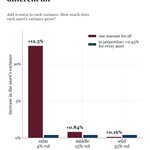
4. The calm asset gets hit the hardest because the charge works like one amount for all: the same small variance number added to every variance. Add 0.0002. For the 4% asset, that is 12.5% more variance. For the 35% asset, 0.16% more. The calm asset looks much riskier so money leaves it - the asset the true answer wants the most! On this menu, one amount for all helped by 0.02 points at most from a 4% start. With the distance picked from one history it slightly hurts. Then true risk rose toward equal weight's 10%. The firs two images show the hit and the money leaving.
5. Change the ruler... now measure each error relative to the vols of its two assets. Under this ruler, the same raw error counts for less between two wild assets, so the "opponent" can push harder there. The charge becomes the distance multiplied by the sum of (weight x vol)^2. That's the same as adding to each variance in proportion to its own size.
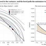
6. The new charge nudges... this charge is smallest when each weight is in inverse proportion to its variance: a lot in the calm asset, a little in the wild ones. Every variance grows by the same percentage, so the calm-to-wild ranking survives and only the correlations shrink. On the menu at the best distance true risk fell from 4% to 3.65% against a true min of 3.28%. From one history via cross-val the distance still gave ~3.7% then it rose toward 5.1%, the risk of inverse-variance weights (pic 3 has both rulers).
7. Both of the uncertainty sets say the true grid is within a set distance of mine, they disagree on what counts as big error. The "opponent" charges differently and the nudge points somewhere else. A 'good ruler' nudges in roughly the right direction towards equal weight when the assets look alike and toward inverse-variance weight when calm and wild assets are mixed together.


Some intuition on relation to shrinkage... For a distance uncertainty set, the min-max is shrinkage exactly.
1. The covariance matrix is a grid of numbers, one for each pair of assets. Each number describes how the assets move together. Pair an asset with itself and you get its own variance. Your portfolio's variance adds up every number in the grid, each one multiplied by your weights in its two assets. So the pairs where you hold a lot of both assets count the most.
2. You *do not* trust the grid you estimated. The 'uncertainty set' says "the TRUE grid is somewhere near the one I estimated, within a set distance." Distance is a ruler for grids: take the gap for each pair of assets, square the gaps, add them up, take the square root.
3. Think of the min-max as a game with two players. You pick a portfolio, then an "opponent" picks the worst grid inside the uncertainty set: the one that makes your portfolio look the riskiest. You want the portfolio whose worst case is LEAST bad.
4. The "opponent" has a fixed amount of error to spread over the grid. It does the most damage on the pairs that count the most for you. So its best move copies your own weight pattern, scaled to fit the distance - the most error goes where you hold the most. The damage then comes out simply: the distance times the sum of your squared weights. For a 60/40 portfolio and a distance of 0.03, that is 0.03 * (0.36 + 0.16) = 0.0156. The opponent's grid is still a valid covariance grid, so this worst case can really happen.
5. A common fix doesn't need this game. Add the same small number to every asset's own variance, and leave the rest of the grid alone. That fix is diagonal loading, a standard shrinkage. It adds the small number multiplied by the sum of your squared weights to the variance of any portfolio. That is the same charge the "opponent" makes, for every portfolio. So the illustrative game picks the same portfolio as loading with the distance. The min-max is shrinkage, and the distance is the amount of shrinkage.
6. If your weights add up to 100%, the sum of squared weights is smallest when you spread out evenly. 50/50 gives 0.25+0.25=0.50; 90/10 gives 0.81+0.01=0.82. So the charge taxes lopsided bets and nudges you toward equal weight. More doubt means a bigger distance a harder nudge. In the second picture, with two assets, the safest mix on the estimate is 75/25. A distance of 0.03 moves it to 60/40.
@__paleologo's red book that @0xFaust12 cited states this in §10.2.3. Doubt with a different shape gives a different shrinkage. If you doubt each correlation by a set amount, the charge is that amount times a squared total: add up each holding's size times its vol and then square the sum.

Some intuition on relation to shrinkage... For a distance uncertainty set, the min-max is shrinkage exactly.
1. The covariance matrix is a grid of numbers, one for each pair of assets. Each number describes how the assets move together. Pair an asset with itself and you get its own variance. Your portfolio's variance adds up every number in the grid, each one multiplied by your weights in its two assets. So the pairs where you hold a lot of both assets count the most.
2. You *do not* trust the grid you estimated. The 'uncertainty set' says "the TRUE grid is somewhere near the one I estimated, within a set distance." Distance is a ruler for grids: take the gap for each pair of assets, square the gaps, add them up, take the square root.
3. Think of the min-max as a game with two players. You pick a portfolio, then an "opponent" picks the worst grid inside the uncertainty set: the one that makes your portfolio look the riskiest. You want the portfolio whose worst case is LEAST bad.
4. The "opponent" has a fixed amount of error to spread over the grid. It does the most damage on the pairs that count the most for you. So its best move copies your own weight pattern, scaled to fit the distance - the most error goes where you hold the most. The damage then comes out simply: the distance times the sum of your squared weights. For a 60/40 portfolio and a distance of 0.03, that is 0.03 * (0.36 + 0.16) = 0.0156. The opponent's grid is still a valid covariance grid, so this worst case can really happen.
5. A common fix doesn't need this game. Add the same small number to every asset's own variance, and leave the rest of the grid alone. That fix is diagonal loading, a standard shrinkage. It adds the small number multiplied by the sum of your squared weights to the variance of any portfolio. That is the same charge the "opponent" makes, for every portfolio. So the illustrative game picks the same portfolio as loading with the distance. The min-max is shrinkage, and the distance is the amount of shrinkage.
6. If your weights add up to 100%, the sum of squared weights is smallest when you spread out evenly. 50/50 gives 0.25+0.25=0.50; 90/10 gives 0.81+0.01=0.82. So the charge taxes lopsided bets and nudges you toward equal weight. More doubt means a bigger distance a harder nudge. In the second picture, with two assets, the safest mix on the estimate is 75/25. A distance of 0.03 moves it to 60/40.
@__paleologo's red book that @0xFaust12 cited states this in §10.2.3. Doubt with a different shape gives a different shrinkage. If you doubt each correlation by a set amount, the charge is that amount times a squared total: add up each holding's size times its vol and then square the sum.

So the solution I was getting at does relate to shrinkage, yes.
We know that once you optimize over Σ̂ the optimizer is now actively selecting on the noise. For a fixed portfolio, σ̂²(w) = w′Σ̂w can be unbiased on average, but once we solve ŵ = argmin_{w∈F} w′Σ̂w we have searched the feasible region and picked the portfolio where the covariance error happened to make risk look "cheapest," which sounds like the problem you mentioned originally.
What came to mind for me is the section from @__paleologo EQI chapter 10 on evaluating a chosen portfolio against plausible errors in the parameters rather than taking the point estimate literally. The book does this explicitly with bounded errors in sharpe forecasts and correlations and looks at the worst-case degradation in realized pnl and sharpe. Importantly, it makes the related point that constraints necessarily hurt the optimum if μ and Σ are known, but can IMPROVE realized performance in the face of estimation error (which of course there is) because they stop the optimizer from exploiting the estimated parameters as aggressively. The formulation I had in mind is basically min_{w∈F} max_{Σ∈U} w′Σw, which seeks to select the best portfolio conditional on the model being wrong within some plausible uncertainty set (coincidentally, this is also how MOSEK frames robust portfolio optimization in its cookbook docs.mosek.com/MOSEKPortfoli…).
If we run a quick simulation around this point, we can take 20 statistically identical assets with 60 observations and perform 1000 draws. Since the true covariance structure is symmetric, the true min-var portfolio should be equal weight, right? Equal weight comes back with ~11.6% risk and actually has ~11.6% risk while the naive sample min-var portfolio reports 9.5% risk but has 14.1% true risk. Adding a robustness/regularization term raises reported risk to 10.4% but brings true risk back down to 11.9%. To your original point, the optimizer was just maximizing the covariance errors that were most favorable to the objective we were trying to solve.
The second chart shows the point I was thinking about from EQI chapter 10. If we sweep the robustness parameter ε, we get a frontier where the in-sample optimum gets worse while the realized risk of the selected portfolio gets better. So another way to handle the issue you mention is to give up some apparent in-sample optimality vs. taking the extreme point produced by the most favorable realization of estimation error.
I'm no expert here at all though as I'm still actively learning but this was just another thought that came to mind and could be totally wrong (and you should tell me if it is!)


I find it useful to rebuild major derivations, recompute examples and keep a ledger of things proven vs things cited. A thread with some takeaways
(1/n)
Michaud (1989) says the optimizer is an error maximizer. Scherer states this problem - the optimizer picks assets with high return and low risk or correlation, "exactly the cases where estimation error is likely to be highest".
Every covariance matrix has directions: unit-length mixes of assets from riskiest to calmest. The eigenvalues are the variances along those directions. Estimate the matrix from a sample and the eigenvalues spread out, the riskiest-looking direction looks riskier than it is. The calmest-looking direction looks calmer than it is.
(3/n)
An optimizer that wants low risk piles into calm-looking directions, where the sample understates risk the most, relative to what it reports.
RMT gives us the size of that spread. Take N independent assets with variance 1, so every true eigenvalue is 1. With T observations, the sample eigenvalues still spread from (1 − √(N/T))² to (1 + √(N/T))².
For any matrix and any sample size, the smallest sample eigenvalue sits below the smallest true eigenvalue on average.
(3.1/n)

There is a partial fix: eigenfactor adjustment. (Menchero, Wang & Orr 2012)
Shrinkage helps narrow the gap (moves reported eigenvalues back toward the truth) but it doesnt remove the selection. The optimizer still picks the directions where the remaining error is most favorable. Of course, real books have constraints, long-only & caps act like shrinkage and limit how far the optimizer can chase noise. (Jagannathan & Ma 2003)
We have two questions: "how risky is this portfolio?" and "which portfolio is least risky?"
The first question holds weights fixed and measures one return series, and that estimate is right on average. (its error shrinks like one over the root of the number of observations)
The second question lets the estimate choose the weights, and because every estimate has errors, some mixes of assets look calmer than they are just by luck. The optimizer cannot distinguish betwen what is "real calm" from "lucky calm". It goes to "lucky calm" because the estimate says thats where the cheapest risk is.
as such - the chosen book looks safer than it actually is.
Another (well-known) reminder... risk models are used for estimating volatility of non-optimized portfolios, they are also used for portfolio optimization.
Most techniques for estimating covar matrices work well for one use case or the other, typically not both.
- Menchero, Wang, and Orr (2012)
- Menchero and Ji (2019)
- Shepard (2007/2008)
:D
On the first day of this new quarter let us recall that BL was built "not at all" (Litterman p.76) from a belief that equilibrium forecasts returns. The case for π is about making MVO more well-behaved.
It's a shrinkage case: a sensible center beats raw sample means inside an optimizer.